MACOS 에서 PyTorch 설치하기
![]()
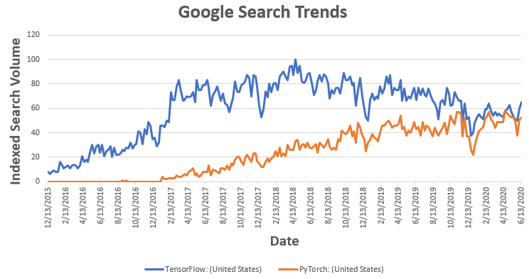
보통 머신러닝/딥러닝 프로젝트를 수행할 시 TensorFlow나 Keras를 많이 사용하였었다. 하지만 PyTorch를 사용하는 사람들이 늘어나면서 나도 개인적으로 설치 방법을 정리해 놓으려고 한다.
TensorFlow vs PyTorch
한 블로그에서 이 두 머신러닝 프레임워크에 대해 잘 정리해 놓은 글이 있어서 이곳에 정리해본다.
Programming API
The Tensorflow API was very cryptic to start with, it almost felt like learning a new programming language, on top of it, it was also very hard to debug due to its static computation graph approach (more on that below). Pytorch (python) API on the other hand is very Pythonic from the start and felt just like writing native Python code and very easy to debug. Tensorflow did a major cleanup of its API with Tensorflow 2.0, and integrated the high level programming API Keras in the main API itself. A combination of these two significantly reduced the cognitive load which one had to undergo while writing Tensorflow code in the past :-) The programming APIs (of TensorFlow and PyTorch) in fact look very similar now, so much that the two are indistinguishable a number of times (see example towards the end)
Computation Graph
Computation graph was a major design difference between the two frameworks to start with. Tensorflow adopted a static Computation Graph approach where one defines the sequence of computation that one wants to do, with placeholder for the data. After that for training / running the model you feed in the data. Static computation graph is great for performance and ability to run on different devices (cpu / gpu / tpu), but is a major pain to debug. Pytorch on the other hand adopted a dynamic computation graph approach, where computations are done line by line as the code is interpreted. This makes it a lot easier to debug the code, and also offers other benefits — example supporting variable length inputs in models like RNN. Fast forward to today, Tensorflow introduced the facility to build dynamic computation graph through its “Eager” mode, and PyTorch allows building of static computational graph, so you kind of have both static/dynamic modes in both the frameworks now.
Distributed Computing
Both the frameworks provided the facility to run on single / multiple / distributed CPUs or GPUs. In earlier days it used to be a pain to get Tensorflow to work on multiple GPUs as one had to manually code and fine tune performance across multiple devices, things have changed since then and now its almost effortless to do distributed computing with both the frameworks. Google made its custom hardware accelerator Tensor Processing Unit (TPU) which can run computation at blazing speed, even a lot faster than GPU, available for 3rd party use in 2018. Since Tensorflow and TPU are both from Google, its far easier to run code on TPUs using Tensorflow as opposed to PyTorch, as PyTorch has a bit of patchy way of working on TPUs using third party libraries like
Deployment / Production
Deployment is something where Tensorflow had a lot of advantage over PyTorch, in part due to better performance due to its Static Computation graph approach, but also due to packages / tools that facilitated quick deployment over cloud, browser or mobile. That’s the reason a lot of companies preferred Tensorflow when it came to production. PyTorch has tried to bridge this gap in version 1.5+ with TorchServe, but its yet to mature
Code Comparison
Its amusing that for a lot of things the APIs are so similar that the codes are almost indistinguishable. Given below are code snippets for the core components on (proverbial “Hello World” problem in Computer Vision) for both Tensorflow and Pytorch, try to guess which one is which The complete Tensorflow and Pytorch code is available at my
Data Loader
# Download the MNIST Data
(x_train, y_train), (x_test, y_test) = mnist.load_data()
x_train, x_test = x_train / 255.0, x_test / 255.0
# Add a channels dimension
x_train = x_train[..., tf.newaxis]
x_test = x_test[..., tf.newaxis]

train_ds = tf.data.Dataset.from_tensor_slices((x_train, y_train)).shuffle(10000).batch(32)
test_ds = tf.data.Dataset.from_tensor_slices((x_test, y_test)).batch(32)
Which one is PyTorch code - above or below?
# Download the MNIST Data and create dataloader
transform = transforms.Compose([transforms.ToTensor()])
xy_train = datasets.MNIST('./', download=True, train=True, transform=transform)
xy_test = datasets.MNIST('./', download=True, train=False, transform=transform)

train_ds = DataLoader(xy_train, batch_size=32, shuffle=True)
test_ds = DataLoader(xy_test, batch_size=32, shuffle=True)
Okay the method to load the data looks a bit different, but I promise it gets similar from here on :-)
Model Definition
# Model Definition
class MyModel(nn.Module):
    def __init__(self):
        super(MyModel, self).__init__()
        self.conv1 = Conv2d(in_channels=1, out_channels=32, kernel_size=3)
        self.flatten = Flatten()
        self.d1 = Linear(21632, 128)
        self.d2 = Linear(128, 10)

    def forward(self, x):
        x = F.relu(self.conv1(x))
        x = self.flatten(x)
        x = F.relu(self.d1(x))
        x = self.d2(x)
        output = F.log_softmax(x, dim=1)
        return output
Which one is PyTorch code - above or below?
# Model Definition
class MyModel(Model):
    def __init__(self):
        super(MyModel, self).__init__()
        self.conv1 = Conv2D(filters=32, kernel_size=3, activation='relu')
        self.flatten = Flatten()
        self.d1 = Dense(128, activation='relu')
        self.d2 = Dense(10)

    def call(self, x):
        x = self.conv1(x)
        x = self.flatten(x)
        x = self.d1(x)
        output = self.d2(x)
        return output
Instantiate Model, Loss, Optimizer
# Instantiate Model, Optimizer, Loss
model = MyModel()
optimizer = Adam()
loss_object = SparseCategoricalCrossentropy(from_logits=True, reduction='sum')
Which one is PyTorch code - above or below?
# Instantiate Model, Optimizer, Loss
model = MyModel()
optimizer = Adam(model.parameters())
loss_object = CrossEntropyLoss(reduction='sum')
Traning Loop
for epoch in range(2):
    # Reset the metrics at the start of the next epoch
    train_loss = 0
    train_n = 0
    for images, labels in train_ds:
        with GradientTape() as tape:
            # training=True is only needed if there are layers with different
            # behavior during training versus inference (e.g. Dropout).
            predictions = model(images, training=True)
            loss = loss_object(labels, predictions)
            train_loss += loss.numpy()
            train_n += labels.shape[0]
        gradients = tape.gradient(loss, model.trainable_variables)
        optimizer.apply_gradients(zip(gradients, model.trainable_variables))
    train_loss /= train_n
Which one is PyTorch code - above or below?
for epoch in range(2):
    # Train
    model.train()
    train_loss = 0
    train_n = 0
    for image, labels in train_ds:
        predictions = model(image).squeeze()
        loss = loss_object(predictions, labels)
        train_loss += loss.item()
        train_n += labels.shape[0]
        loss.backward()
        optimizer.step()
        optimizer.zero_grad()
    train_loss /= train_n
It’s really interesting (and convenient!) how similar the APIs seem to be now.
Environment
내가 설치한 환경은 MAC(Big-Surr) 환경이고 virtalenv를 통해 따로 가상환경을 만들어 놓았다.(Python 3.8.5) 간단하게 pip를 통해 설치가 가능하다. 파이썬 환경에 대한 설명은 생략하도록 하겠다. 공홈에서는 요세미티 이상에서 설치가 가능하다고 하고 Python 3.5 이상을 권장하고 있다.
더욱 더 자세한 내용은 PyTorch 공식 홈페이지 를 참고하자.
Install
대부분 Anaconda 패키지 형태로 설치를 많이 하지만 간단히 아래의 명령어를 통해 설치가 가능하다. 다만 MAC용 바이너리에서는 CUDA를 지원하지 않는다고 한다.
pip install torch torchvision torchaudio
# MacOS Binaries dont support CUDA, install from source if CUDA is needed
Verification
설치가 끝났으면 제대로 설치가 되었는지 확인해 보자.
import torch
x = torch.rand(5, 3)
print(x)
위의 코드를 실행했을 때 아래와 같이 5x3 배열의 형태로 나오면 제대로 설치가 완료된 것이다.(안의 숫자는 다를 수 있음)
tensor([[0.3380, 0.3845, 0.3217],
        [0.8337, 0.9050, 0.2650],
        [0.2979, 0.7141, 0.9069],
        [0.1449, 0.1132, 0.1375],
        [0.4675, 0.3947, 0.1426]])
댓글남기기